AP Biology 5.3 - Mendelian Genetics
This section of the AP Biology curriculum builds on our understanding of heredity and meiosis by introducing Gregor Mendel and Mendel’s laws. The Law of Dominance, the Law of Segregation, and the Law of Independent Assortment create rules for the inheritance of different alleles that allow us to predict the outcome of various matings as long as a few of the alleles are known. In this section, we’ll also learn how to use Punnett squares to predict the outcomes of different crosses. Specifically, we’ll see how Punnett squares can be used to predict the genotypic ratio and phenotypic ratio of offspring in monohybrid crosses, dihybrid crosses, and beyond. We’ll also see how a test cross can be used to determine the alleles carried by an organism with an unknown genotype. Finally, we’ll see how we can determine whether or not our hypotheses about genetic outcomes are supported by the observations we make of actual populations using the chi-squared analysis!
Video Tutorial
The following video summarizes the most important aspects of this topic!
To watch more tutorial videos like this, please click here to see our full Youtube Channel!
Resources for this Standard
For Students & Teachers
- Overview & Video Tutorial (This article)
- Quick Test Prep
- Crossword Puzzle
For Teachers Only
ENDURING UNDERSTANDING
EVO-2
Organisms are linked by lines of descent from common ancestry.
IST-1
Heritable information provides for continuity of life.
LEARNING OBJECTIVE
EVO-2.A
Explain how shared, conserved, fundamental processes and features support the concept of common ancestry for all organisms.
IST-1.I
Explain the inheritance of genes and traits as described by Mendel’s laws.
ESSENTIAL KNOWLEDGE
EVO-2.A.1
DNA and RNA are carriers of genetic information.
EVO-2.A.2
Ribosomes are found in all forms of life.
EVO-2.A.3
Major features of the genetic code are shared by all modern living systems.
EVO-2.A.4
Core metabolic pathways are conserved across all currently recognized domains.
IST-1.I.1
Mendel’s laws of segregation and independent assortment can be applied to genes that are on different chromosomes.
IST-1.I.2
Fertilization involves the fusion of two haploid gametes, restoring the diploid number of chromosomes and increasing genetic variation in populations by creating new combinations of alleles in the zygote —
- Rules of probability can be applied to analyze passage of single-gene traits from parent to offspring.
- The pattern of inheritance (monohybrid, dihybrid, sex-linked, and genetically linked genes) can often be predicted from data, including pedigree, that give the parent genotype/phenotype and the offspring genotypes/phenotypes.
RELEVANT EQUATIONS
Laws of Probability-
If A and B are mutually exclusive, then:
P(A or B) = P(A) + P(B)
If A and B are independent, then:
P(A and B) = P(A) x P(B)
5.3 Mendelian Genetics Overview
Believe it or not, the first insight humans had into how genetics work came from the dedicated work of a Catholic friar experimenting and observing the traits of pea plants. Now considered the father of genetics, Gregor Mendel started with the common knowledge that crossbreeding plants and animals could lead to offspring with different traits. By carefully crossing pea plants with specific traits, Mendel found that the offspring often had predictable ratios of various traits. Working backward from this, Mendel developed a number of rules that apply to how traits are inherited from parents to offspring. We call these rules “Mendel’s Laws.”
Mendelian genetics is the study of Mendel’s laws and the probability that different genes will be inherited in the offspring created by two sexually-reproducing organisms. While our understanding of genetics has expanded far beyond Mendel (into non-Mendelian genetics), we can use Mendel’s Laws to predict how offspring will inherit many different kinds of traits – simply based on how genes are sorted during meiosis and recombined during fertilization. Mendelian genetics and probability testing using chi-squared analysis will definitely be on the AP test. So, stick with us as we cover everything you need to know about Mendelian Genetics!
Before we can understand Mendel’s laws, we have to understand a little bit about genetics and evolution. First, even though Gregor Mendel was a lowly friar who was born in the 1820s, even he had a basic understanding of heredity. Farmers, for thousands of years, have understood that offspring have a chance of inheriting the traits of their parents. This is how early humans selectively bred everything from livestock to the crops we survived on. Though Gregor had no idea how these traits were passed on a molecular level, he had the basic foundational knowledge that traits were inherited from parents.
While this was all that Gregor Mendel needed to know to get started, there are several other things we know now that will be incredibly helpful as we start to discuss Mendel’s Laws and Heredity. We now know that genetic information is carried by two molecules, DNA and RNA.
DNA carries the information, is transcribed into an RNA molecule that can leave the nucleus, and this RNA molecule is translated into a protein molecule via a ribosome. Protein molecules are like cellular machines that create functions within cells, and therefore create the outward traits (called phenotypes) that Mendel was observing.
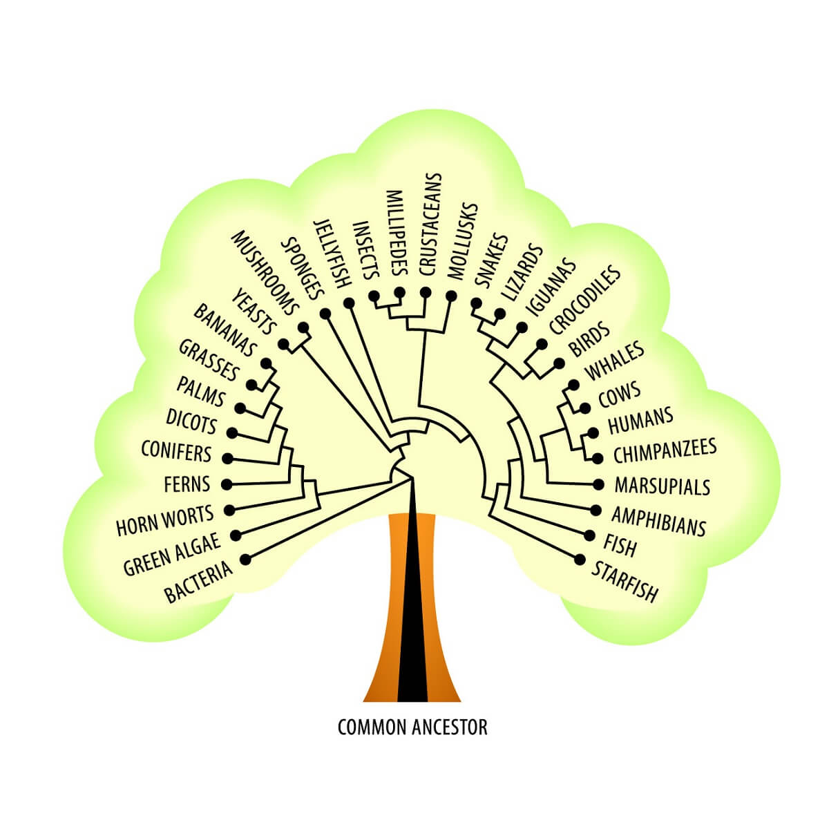
We also know that these ribosomes are found across all domains of life – from the simplest bacterial cells to the cells of more complex, multicellular eukaryotes. Not only do all domains of life share this basic foundational mechanism for protein creation, but they also share many other metabolic pathways – such as creating and using carbohydrates, synthesizing phospholipids for cell membranes, and many other core functions. All of these facts suggest a continuity of life from a single, shared common ancestor that likely arose billions of years ago! With all of this in mind, let’s take a look at Mendelian Genetics and the laws that Mendel uncovered.
Think about this… while some traits and conditions are influenced by a large number of genes, some diseases can be caused by a single genetic mutation. These genetic diseases can be detrimental. However, we can also easily predict whether two parents have the potential to pass these genetic diseases onto their children using simple and relatively cheap genetic tests. As we start to look at the probability of inheritance using Mendel’s Laws, keep these genetic conditions in mind!
In starting his pea plant experiments, Mendel understood two basic things about the pea plants he was working with. He understood that pea plants reproduced by producing pollen in the male stamen organs, which travels to the female stigma organ. Since each pea plant flower has both male and female parts, a single flower can reproduce by itself in a process known as selfing. In order to conduct his experiments, Mendel prevented this process by removing the stamens from one of the plants he wanted to reproduce. Using a paintbrush, he carefully transferred pollen from one flower to the other, ensuring that the first flower was pollinated by a plant of his choice.

In one of Mendel’s most famous and important experiments, he crossed a line of plants that only produced purple flowers with a line of plants that only produced white flowers. When he collected and planted the peas, he found that all of the plants had purple flowers. Though the parental generation had white and purple flowers, the next generation (denoted the F1 generation) consisted of only purple flowers. However, Mendel found that if he crossed two of these F1 plants into a new generation (the F2, generation) at least 1/4th of the plants would have white flowers.
This is how Mendel developed his first law, the Law of Dominance. This law states that some alleles (like the allele that creates purple flowers) can cover up other alleles (like the allele that creates white flowers) in a heterozygous organism that has 1 of each allele. However, we have expanded on the Law of Dominance to include more than just complete dominance. Incomplete dominance is where the heterozygote is a completely new phenotype, such as a pink flower produced by the combination of a red homozygote and a white homozygote. Codominance is where both homozygous traits are expressed in the heterozygote.
But, what about Mendel’s second and third laws? The Law of Segregation states that different alleles are separated into different gametes, allowing for dominant and recessive alleles to be inherited separately. The law of segregation can also be inferred from Mendel’s most famous flower color experiment. Since the F2 generation contained some white flowers but the previous generation didn’t, it must be assumed that the alleles for white flowers were hiding in the F1 generation and became separated from the dominant purple alleles before they were inherited.
By contrast, the Law of Independent Assortment can only be seen when you look at two different traits at the same time. This law states that different genes are inherited independently from one another. For example, the gene controlling a plant’s flower color is not connected to the gene controlling pod color. A plant can inherit purple flowers and yellow pods, white flowers and green pods, or any other combination of the two traits. While Mendel got lucky and chose many traits that were not physically linked, we know now that the Law of Independent Assortment is only true of genes that are located on separate chromosomes. If genes are located on the same chromosome, there is actually a good chance that they will be inherited together. These processes were covered previously in section 5.2 if you need a refresher.
It wasn’t until nearly 50 years after Mendel’s experiments that another scientist – Reginald Crundall Punnett – devised a way to determine the probability that an offspring would receive a given allele in a mating between two organisms. This tool was the Punnett square.
The Punnett square is a simple tool that takes what we know about meiosis and sexual reproduction and puts it in a table to predict the outcome of a genetic cross. When considering 1 trait, the Punnett square has 4 squares – a vertical column for each copy of each paternal allele, and a horizontal row for each copy of each maternal allele. Then, you simply distribute the alleles to each box, which represents a potential fertilization event between gametes carrying these alleles. This gives us the genotype of each potential offspring.
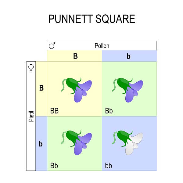
In the case of this trait – flower color in pea plants – there are two alleles. The “B” allele shows complete dominance over the “b” allele. So, any squares with a “B” will have a purple phenotype. This includes both the homozygous dominant square and the heterozygous squares. Any squares that are homozygous recessive (two “b” alleles) will be white.
What the Punnett square really shows us is the probability of each genotype and phenotype for different types of crosses. This is a monohybrid cross, since both parents are hybrids (or heterozygotes) and we are only looking at a single trait. All monohybrid crosses have the same genotypic ratio. This ratio is always 1 homozygous dominant to 2 heterozygotes to 1 homozygous recessive. The phenotypic ratio, on the other hand, is only the same if alleles showing complete dominance are involved. In this case, 3 of 4 times the offspring will have the dominant phenotype, while 1 of 4 times the offspring will have the recessive phenotype. This gives us the probability of each phenotype and genotype, regardless of how many individual offspring are created by each cross.
Plus, the general idea of a Punnett square can be expanded simply by adding more squares. Let’s take a look at a dihybrid cross – a cross between organisms that are heterozygous for two traits showing complete dominance. Just like before, each row and column in this expanded Punnett square shows a potential gamete and each square is a hypothetical fertilization event between two gametes. This Punnett square can give us the probability of an offspring receiving a specific combination of traits. While anything above a trihybrid cross starts to become too difficult by hand, computers can easily handle the complex calculations and geneticists can use computerized Punnett squares to predict any number of different traits.
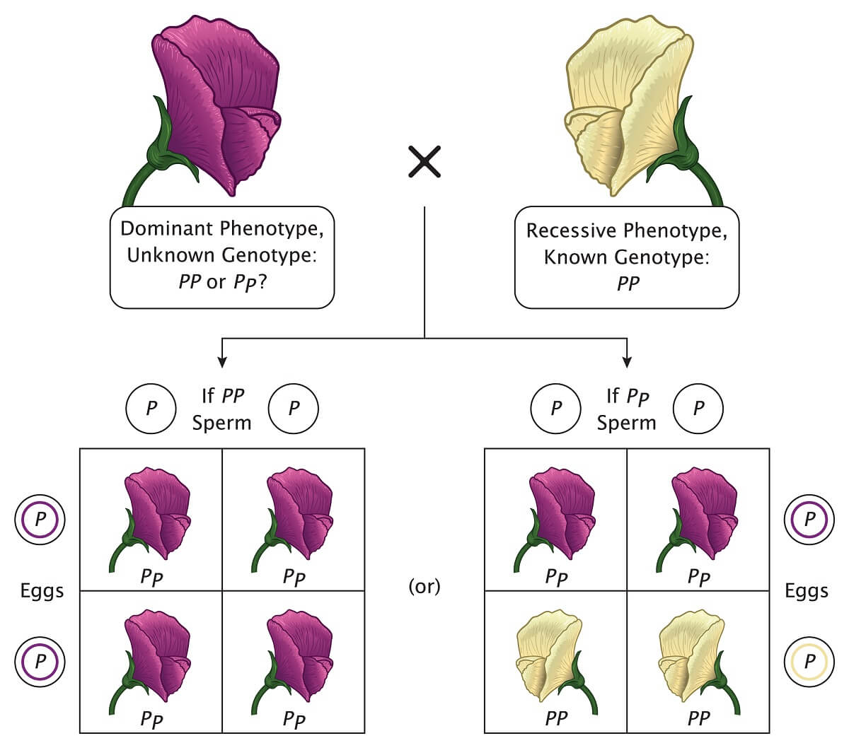
Plus, the Punnett square is an easy way to figure out which genes an unknown organism carries through a test cross. Since we always know the genotype of organisms with a recessive phenotype, we can cross a recessive phenotype with a plant that has an unknown genotype. If the offspring show the recessive phenotype, we know that the unknown genotype contained one recessive allele. If the offspring only show the dominant phenotype, we know that the unknown genotype was homozygous dominant.
Consider a gene for flower color. We hypothesize that this trait shows complete dominance. Using a Punnett square, we can easily predict a phenotypic ratio of 3:1 – 3 dominant phenotypes and 1 recessive phenotype. So, if we were to measure 100 offspring, we should expect 75 dominant phenotypes and 25 recessive phenotypes. However, due to random chance, we also expect there to be at least some deviation from these “perfect” Mendelian ratios since the alleles every gamete gets is like flipping a coin. Let’s say that after observing 100 offspring we find 70 dominant phenotypes and 30 recessive phenotypes. So, how do we know whether or not these deviations support our hypothesis?
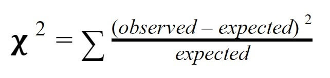
This is where chi-squared testing becomes useful. Chi-squared testing is a simple statistical technique that can tell us whether or not our observations support a particular hypothesis or expected value. To measure chi-squared, we subtract the expected value from the observed value, square this number, then divide by the expected value for each “class” (in this case each phenotype). Then, we add together all of the classes to get the overall chi-squared value. Formally, the formula is read: “Chi-squared equals the sum of observed values minus expected values, squared, divided by expected values for each class.”
So, to calculate the chi-squared value for our particular experiment, we simply need to calculate observed minus expected, squared, divided by expected for each class, then add them together. When we do so, we find our chi-squared value is 1.33. But, what does this mean?
To understand if our chi-squared value supports our hypothesis, we have to compare our chi-squared value to a critical values table. First, we calculate how many degrees of freedom are present in our chi-squared value. The “degrees of freedom” is simply the number of classes minus one. Since we had only two classes, we have only 1 degree of freedom. Then, we find where our chi-squared value fits in the table. 1.33 fits in the table between the P-values of 0.5 and 0.1. This means that between 50% and 10% of the time we would expect deviations as large as we observed. Since most scientists agree that P-values above 5% signal support for a hypothesis, we can accept our observations as support for our hypothesis.
Keep in mind that you can test almost any number of classes with a chi-squared analysis. The AP test will likely have you calculate something more complicated than this, so be sure to take the quiz in the Resources section to see if you are up to the task!