This standard focuses on how we can show evolution through mathematical models. More specifically, the standard aims to show how heritable traits can increase within a population if they are beneficial to survival and reproduction.

Resources for this Standard:

• Overview (This article)
• Quick Concept Quiz

Coming soon!

Here’s the Actual Standard:

Apply concepts of statistics and probability to support explanations that organisms with an advantageous heritable trait tend to increase in proportion to organisms lacking this trait.

Standard Breakdown

There are many ways to use statistics and probability to see evolution in action.

Distribution of Traits

The easiest way to visualize traits within a population is to plot the frequency of each trait compared to all traits. What we find when we do this is that most traits fall into a normal distribution, as seen below:

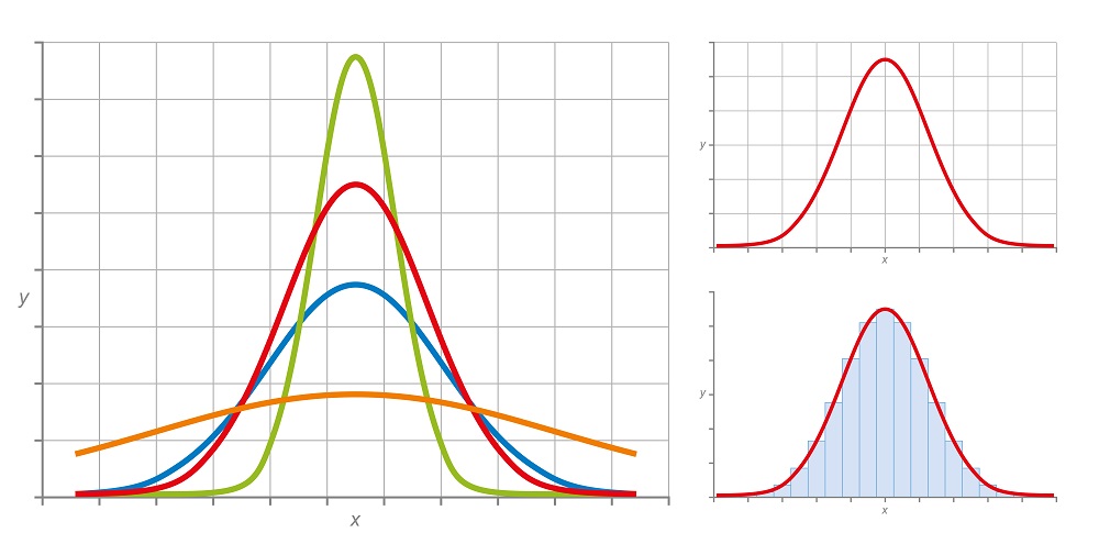
Statistically, we can break traits into two categories: discrete and continuous traits. Discrete traits, such as hair color, can be categorized into discrete categories, like the graph on the lower right of the image above. While individual organisms fall into discrete categories, the overall distribution of the variation remains the same. Continuous traits, such as height, do not clearly fall into different categories, and each individual can be added to a continuous distribution, such as the graph on the upper right of the image.

Further, we can estimate the variation present within a population by looking and the width – or breadth – of the normal distribution. The green line represents a population with very little variability, whereas the orange line represents a trait with a much higher level of variation spread more evenly across all versions of the trait.

Trait Distribution over Time

To really see evolution in action, we have to look at the distribution of traits over time. Essentially, this is a mathematical proof that populations evolve over time – as seen in the graphs below:

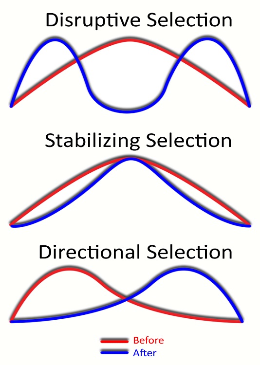
Directional selection happens when the mean value for the trait shifts one direction or another. This could mean the population is getting taller, heavier, or is moving toward one end of the color spectrum. A good example of directional selection is the evolution of flippers in whales and dolphins.

Stabilizing selection happens when there are selective pressures on the extreme variations of a trait. It can be thought of as “Goldilocks selection” in that it selects for the trait that is “just right” – not too hot or too cold. An example of stabilizing selection could be the color of a population of mice. If white mice and black mice get predated at higher rates, gray mice might be selected for because they have the best camouflage.

Disruptive selection happens when a new selective pressure targets the mean trait in a population. For example, if a new predator in an environment eats only gray mice, black mice and white mice will both increase in abundance. Disruptive selection, brought on by a wide variety of selective forces on a large number of traits, can ultimately lead to a speciation event – when the population splits based on a disrupted trait it can stop interbreeding and form new species.

A little clarification:

The standard contains this clarification statement:

Emphasis is on analyzing shifts in the numerical distribution of traits and using these shifts as evidence to support explanations.

Let’s look at this clarification a little closer:

Shifts in Numerical Distribution

As seen above, we can directly monitor these shifts in the numerical distribution of variants in a trait. An important note on this point is that is important for students to understand what each axis represents.

The Y-axis is a measure of abundance – or how frequently a trait appears in a population. If the entire population has been measured this could be an actual number. However, most of the time this abundance is simply a percentage of the population, based on capture/recapture studies done in populations. (Essentially, a number of organisms are captured, traits documented, each organism is marked, and then released back into the environment. Sometime later, another sample of the same number of organisms is collected. Based on the ratio of marked individuals to unmarked individuals, the total size of a population can be estimated, as well as the abundance of different variations.) Based on changes in the abundance of different traits, we can “measure” evolution as it happens.

The X-axis can represent many different things, based on how it is labeled. With discrete traits, the category is often labeled – such as green eyes, brown eyes, blue eyes – or it is a simple number line representing the quantification of a continuous trait – such as measuring each student’s exact height. Plus, it should be noted that most traits are no truly discrete or truly continuous. Most traits are a combination of genetics and the environment. Genetics by themselves are discrete traits – each nucleotide position within the DNA could be considered a trait and there are only 4 nucleotides. However, as genetics interact with the environment a massive amount of variation can often be seen between identical DNA that has experienced different conditions.

What to Avoid

This NGSS standard also contains the following Assessment Boundary:

Assessment is limited to basic statistical and graphical analysis. Assessment does not include allele frequency calculations.

Here’s a little more specificity on what that means:

Statistical and Graphical Analysis:

Assessment should focus on interpreting what a graph means, and how the abundance measurements in each trait can be used to statistically quantify traits in a population, essentially what was covered above.

Allele Frequency Calculations:

Allele frequency is a measurement of how often a specific allele is found within a population. For simplicity, this standard focuses only on phenotypes (visible/measurable traits). Looking at allele frequencies, or the actual variation within the genome complicates how this relates to evolution. Allele frequencies, and their importance in evolution, are covered in other standards.